Don't fear the smoother

Years ago when I first started at Cyentia, I was going over some analysis with the great Jay Jacobs and had produced a scatter plot. The points didn’t show a clear trend but Jay suggested “drop a geom_smooth in there and see if there is a trend”. I scoffed. I sneered. “A non-parametric smoothed regression? How were we supposed to interpret the swoops and curves?” Jay probably rolled his eyes and we moved on.

Friends, let me say that reaction was, as most anti-non-parametric bigotry is, born out of ignorance. And of course that which we don’t understand, we tend to fear. But after some deep soul searching (and some literature review) I’ve come to embrace and love smoothed regression. Let me tell you: it’s pretty great.

So great in fact that we used it extensively in the most recent Veracode State of Software Security Volume 12 report. Check out the beautiful swooping lines in Figure 5 reproduced below.

Beautiful data, beautiful smoothed regression.

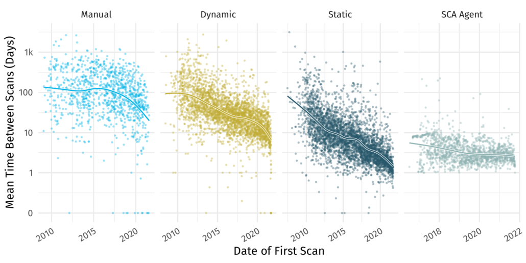
For those that don’t know, Veracode provides tools that help developers identify and fix flaws in their software throughout the development pipeline. Here we show different ways to identify flaws in a codebase through 4 scan types. Each point here is an application that was scanned by a particular scan type. The figure shows the time between scans for that application over time.

It shows the precipitous decline of time between scans across all different types. I won’t pick it apart here, go to the full report for commentary, but the main takeaway is there is a decline in scan cadence for all different types of scans. Additionally there seems to be some speedup in decline for things like manual scanning starting in mid 2017.

So how can we draw such lovely regression lines? Follow me down the road to understanding generalized additive models(GAMs).

Line charts and interpolation

As you no doubt remember from primary school, the shortest distance between two points is a straight line¹. But what happens when we have more than one point and they don’t quite all line up? Well we tend to just connect those points with little segments of lines anyway.

How we usually go about interpolating between lines.

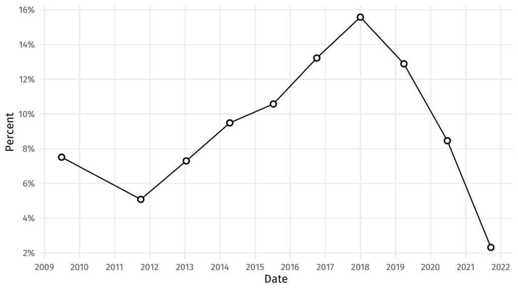
But, as the great Robert Kosara has recently pointed out, it’s somewhat silly to think that when we have discrete samples of data we should interpolate the points in between linearly with sharp transitions at those endpoints. This is especially true in the figure above, where we are looking at a percentage change over time. It’s likely that the percentage changed more smoothly than that. So how can we represent that smooth transition? Enter the spline.

From drafting to interpolating

Data analysts are not the first ones to need a method of drawing nice smooth curves. The term spline comes from a drafting tool used to create smooth curves. However, when we’re dealing with data firmly embedded in the memory of a computer, long flexible strips of wood (or plastic nowadays) aren’t going to do us much good. Thankfully, Isaac Jacob Schoenberg came along in 1949 and laid down the mathematical foundation for most of what we know about interpolation today. In particular, he noted that, with a certain functional form, we could create a relatively simple mathematical object that closely approximates the physical characteristics of the long strips of wood/plastic used by drafters. And thus cubic splines were born.

As much as it would delight me to, I won’t go into the mathematical detail here. Suffice to say that there are a plethora of software packages that will take some data points and output points interpolated in between using cubic splines². So let’s do that with our graph above and see what it looks like.

The same points, now nicely smoothed.

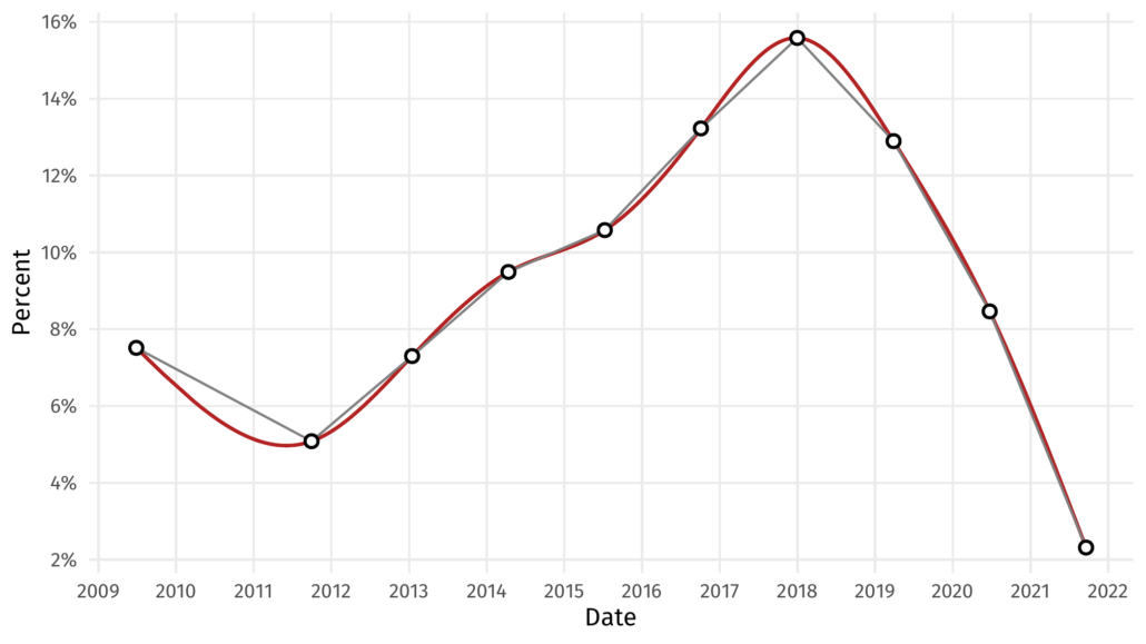
That red line provides a more realistic version of the data between the points than linear interpolation might.

From smooth interpolation to smoothed regression

OK, but what if we have more than 10 data points, and what if those points are messy? Like this

How do we smooth this many points?

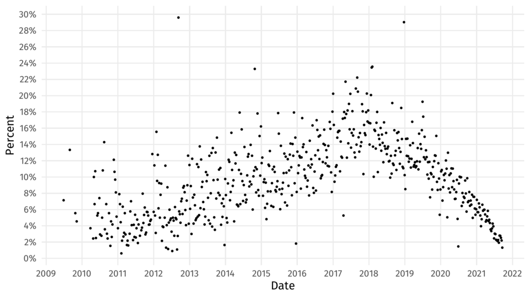
Certainly we can’t interpolate through every single point on that figure. Moreover, something like linear regression is going to fail us because the data clearly rises and falls over time. We could try a high degree polynomial regression, but the non-symmetric nature of this data is likely not going to give us a good fit. Polynomial regression is also bad for many reasons, but that’s a story for another blog post.

What would be great is if we could pick some points that could act as anchor points for a spline through the data. This is exactly the goal of Generalized Additive Models, a type of smoothed regression³. In broad strokes, Generalized additive models place a handful (the number is sometimes user defined, sometimes algorithmically selected) of points along the horizontal axis, use an optimization algorithm that then locates their vertical position in much the same way the slope and intercept are selected for linear models. 

If you are a model nerd like me, your brain is already spinning. There are so many ways to adapt this to various data situations! There is indeed a whole world of smoothed regression out there, but rather than tumbling down that rabbit hole, let’s talk about why this is useful.

Analyzing multi-language applications with smoothed regression

So where did that cryptic data we’ve been using come from anyway? Diligent readers might recognize it as figure 3 from the Veracode State of Software Security Volume 12 report. Here it is reproduced in its entirety with a smoothed line.

Where did all this data come from anyway? Application scans over time with a smoothed regression

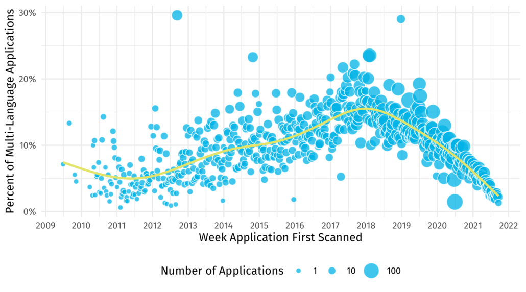
Whereas it might be difficult to draw conclusions about the ups and downs of the data, the smoother gives us more precise insight. For example, the ‘peak’ of multi-language applications is difficult to discern from the points but the smoother tells us it is nearly exactly the beginning of 2018. Without the smooth I might have guessed mid-2017. We can also perceive that the rise of multi-language applications was at a slower rate than its decline post 2018.

So next time you are looking at a scatter plot and want to understand how the data might be related, consider adding a smoothed regression rather than a plain old straight line!

¹ At least in Euclidean space.

² And other types of splines. Too many to talk about here!

³ This is distinct from LOESS regression, which is also often called smoothed regression or local regression. Yet another blog post.