Gain Confidence with Confidence Intervals

I’ll be honest, I have a love/hate relationship with confidence intervals. On one hand, they are indispensable — confidence intervals put a (quantified) frame around outcomes and helps us understand the “strength” of our observations.  On the other hand, they can be just plain confusing and may create more confusion for many readers. Explaining why observing 42% of some phenomenon may not  be an increase from the last measurement of 38% can make for some very puzzled looks.  Since we want the research we do at Cyentia to be as honest and clear as possible, you will come across confidence intervals in our published work.  I hope to demystify these ranges and help you get an intuitive understanding of what confidence intervals are.  

A Quick Example

Let’s say I want to study if a coin is fair (meaning there is a 50% chance of heads coming up).  To test this, let’s say I flipped the coin 10 times and I got 4 heads.  That is a 40% chance of heads, not 50%, so should I claim the coin is not fair?  I think most people understand that 4 heads out of 10 flips isn’t crazy for a fair coin and it is not enough proof to challenge the coin. However, what if I flip the coin 1000 times and get 400 heads?  That’s the same calculated 40% chance, but it feels different doesn’t it?  Would you feel more confident about challenging the coin now?  What’s the difference between estimating 40% chance of heads from 10 flips versus 1000 flips?

I know that estimating if a coin is fair or not may never come up in your personal or professional career, but coin flips and other games of chance are excellent proxies for problems you do care about.  Assessing the rate of fraudulent transactions or malware infections, for instance, will use the same exact math as coin flips.  Studying games of chance is nice because the true probabilities are generally known, so the math and approaches can be (dis)proven.  Having said that, let’s try an analogy with a touch of realism.

Tracking Botnet Prevalence

Let’s say we want to study the infection rate of different malware families, and let’s time bound it over the last 30 days.  Understanding the infection rate is helpful because it will translate directly into a forward looking probability of infection, which then may drive spending decisions. For the sake of simplicity though, let’s ask a simple and clear question:

What proportion of organizations have detected/discovered a specific botnet in their environment in the last 30 days?

Again, this is a hypothetical.  But to start out, let’s suspend reality for a moment and assume that I’ve checked with every organization and 20% of them have seen our hypothetical botnet in the last 30 days, so the statistic we are trying to discover is that 20%. But in reality, nobody has the time or resources to check with every organization.  We always have to settle for less than all the companies; we have to draw a sample. Sampling introduces uncertainty and this is where confidence intervals help out–  they help us understand how much uncertainty the sampling has introduced.

Okay, let’s say we’re on a budget and we can only contact 100 organizations, and let’s say 26 of those say that they’ve seen the botnet in the last 30 days. The 26% we observed seems quite a distance from the 20% we should see, right?  Well, when we consider the basic 95% confidence interval¹, our 26% now becomes a range from 17.4% to 34.6%.  The simple explanation of this range is that the true value (20% in our case) has a very good chance (95%) of being between those two numbers.  But never say that explanation out loud, even though it’s relatively simple and intuitive, because it’s technically wrong.  But I’m telling you to think of it that way because the correct explanation is super confusing: if we repeat the experiment multiple times, 95% of the confidence intervals we generate from those experiments will contain the true value.  The difference between the two explanations is just too subtle to matter in practical applications so I’ll say remember the correct one, but honestly, just simplify it to the easy one.  

Now let’s say some time has passed and we want to update our estimates and see what’s changed. We run another study, but this time we reach out to 250 companies and 46 of them (18.4%) say they’ve seen the botnet. We’ve gone from 26% in the first study to 18.4% in the follow up study.  That sure seems like a big drop, but when we look at the 95% confidence interval it’s 13.6% to 23.3%.  And let’s look at the confidence intervals from the first study compared to the second.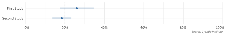

I added a vertical line at the “true value” of 20%.  But notice a couple of things about this plot.  First and most importantly, the two ranges overlap.  If two confidence intervals overlap, you should refrain from making the claim they are different.  This is very difficult for people to accept though since the first study showed an infection rate of 26%, the second study showed a rate of 18.4%, and yet we should not claim the infection rate has dropped.  This is because the drop could easily be explained by sampling error.  How much of the difference is from taking a sample and how much is a change in the true value?  That’s the challenge, and with the data we have, we just don’t know and must be careful about claiming things have changed.  And that’s an important distinction. It doesn’t mean that the underlying infection rate didn’t shift– it means that the sample size was just too small to detect any difference.

Which brings us to the second thing to observe, notice how the range for the second study is more compact than the first study?  The first study had 100 companies while the second study had 250. Larger samples have tighter confidence intervals and larger samples can therefore detect smaller changes.  When we use confidence intervals there is no sample size that is too small.  What if we asked a single company, and they hadn’t seen the botnet?  Using a slightly more advanced confidence interval, we could estimate that the true infection rate is between 0% and 79%.  While that probably is not helpful, we could still use a single sample like that show that it’s unlikely the rate of infection is above 80%.  If we ask 5 companies and none have seen the botnet, we could estimate the infection rate is less than 50% and no more than half of companies have detected the botnet in the last 30 days.  The more samples we can collect the more we can tighten up our confidence interval.  Hopefully you are beginning to see how confidence intervals can help quantify the “strength” of our observations.

Driving this home

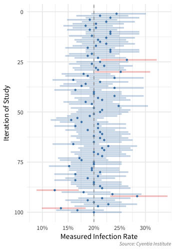
Since we suspended reality and know that there is a 20% chance of seeing this botnet, we can simulate multiple different studies. So let’s sample 250 companies, but let’s repeat that study 100 times.  For each of the 100 studies, the plot shows the point estimate with a solid dot (which is the number of infections divided by the number of companies, 250 in this case).  I also am projecting the 95% confidence interval by showing the bar around the point.  If the confidence interval does not contain the true value (20% in this case as shown by the vertical dashed line), I made the confidence bar red to stand out.  Note these are not invalid samples, just that at 95% confidence, there is a small random chance the true value is not in the range. This means we should expect around 5 studies out of 100 to not contain the true value.

As you look at the plot to the right, try picking out any single study and envision that is the only study you conducted, how confident (the bar) are you around the result?  Pick out two studies and while you compare them think about they are both doing their best to measure the same exact thing.  Different outcomes like these are unavoidable and should be expected, but the good news is the difference are quantifiable.  But think about it – if you didn’t look at the confidence interval, how easy is it to be fooled into thinking the two studies are showing a change?  Mistakingly seeing change happens far more then it should and ridiculous claims of differences make headlines without any account for sampling error.

Even though confidence intervals can be confusing, take some time with them and get to know them, they are showing up in the research we Cyentia Institute research!

¹Note, I generically talk about confidence intervals here, but I am focusing on confidence intervals around a proportion.  Another popular use of confidence intervals is around the estimation of the mean but I rarely end up using that in practice.  In the R language I use the binom package for proportions.  The “binom.asymp” is the confidence interval they teach in basic stats courses, but that’s been shown to be overconfident in smaller proportions and with proportions that approach zero or one, for most applications I’ll leverage the wilson interval. For most decisions the differences between the methods aren’t going to shift outcomes. If you are looking at Cyentia Institute research, the confidence interval will be a 95% confidence interval using the wilson method unless explicitly stated otherwise.