Application Security and Burstiness

It has been a while since my last (and first real) post. We’ve been busy, and so, in the interest of getting back into the swing of blogging I’d like to talk about a fun bit of analysis on application security we did in a fresh off the presses report.

In our latest collaboration with Veracode on the State of Software Security Volume 10, we analyzed more than 85,000 applications to try to better understand application security. We sliced things every which way:

• What percentage of security flaws are fixed?
• How long does it take to fix the typical flaw? And what do we mean by “typical”?
• What contributes to the accumulation of security debt?
• How do these things vary by: scans per year, language, flaw type, severity, exploitability, industry and even geographic region?

All of the above provide insight into the development process and the landscape of application security. One topic stood out to me though and that was the concept of ‘Burstiness’. Let’s dive in and talk about measuring burstiness and how it can change application security.

What does burstiness look like?

Figure 11 gives a good visual display of burstiness

Figure 11 Cadence of security scanning across a sample of applications

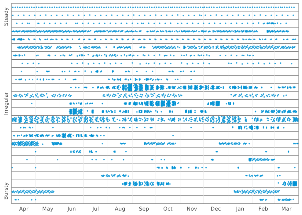
From the figure it’s pretty clear that application developers vary widely in scanning behavior. Some begin (or end) each day with a nice fresh clean scan of their applications, shining a light on its flaws or lack thereof. This might indicate a more Agile approach. In contrast, some developers clearly code madly for months on end without scanning and then scan repeatedly as they fix up all the accumulated security debt. Sounds like a Waterfall approach to me. And of course some applications are developed somewhere in between.

In the figure we label these ‘Steady’, ‘Bursty’, and ‘Irregular’, respectively. But other than eyeballing the graph how do we quantify how “bursty” something is? Enter the Fano factor.

Fano Factor

The Fano factor was developed by Italian American physicist Ugo Fano. Besides having a fun name to say, Dr. Fano made contributions to numerous fields including molecular and radiological physics. The Fano factor most frequently arises as a corrective constant in particle detection in various different elements. It is also frequently used as a measure of burstiness in spikes in neural activity. Interestingly, its calculation and exact value for different applications is not without controversy.

The Fano factor is the ratio of variance of a dataset to its mean. It allows us to take the series of dots in Figure 11 and assign a number. More specifically, we calculate the Fano factor on the time in between scans. Steady scanning means a low variance in the time between scans and a low factor. Long waits between scans followed by rapid scans result in high variance and potentially low means resulting in a high factor. Using the Fano factor we don’t have to manually eyeball and categorize each applications scanning cadence. As a results, we can take the various Fano factors, break them into sensible categories, and then use those categories to measure the effect on things like security debt.

For example,  here is that same figure with each applications Fano factor annotated in Veracode pink.

Figure 11B Cadence of security scanning across a sample of applications with annotated Fano factors

Fano Factor and Application Security

So how does scanning frequency affect things like security debt? Well let’s say “don’t go chasing waterfalls”, here’s figure 36 from the report.

Figure 36 Comparison of fix capacity and security debt by scan cadence

As you can see, applications with a steady scanning cadence tend to accumulate less security debt as the application ages. In contrast, those bursty scanners that wait months tend to accumulate large amounts of debt as the application ages. The SoSS X report examined more than just security debt. Another important aspect was how quickly and completely flaws in applications are addressed.

Figure A Survival curves for applications with various scanning cadences.

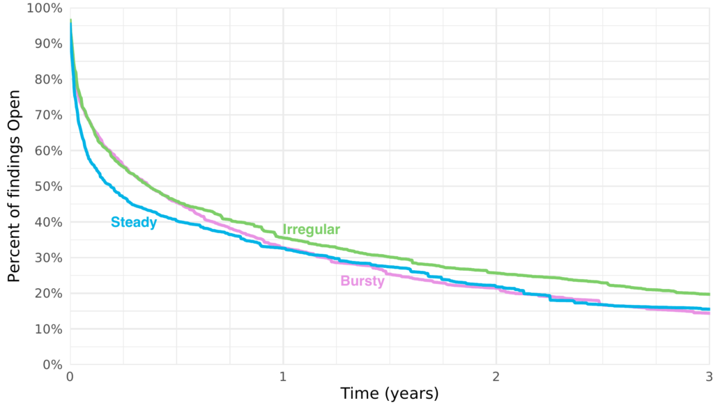
Figure A presents survival curves for flaws found in applications with bursty, irregular, and steady scanning cadences. It mirrors the results we saw in Figure 36 in the first nine months of application age. Interestingly, in the long term, bursty and steady scanning converge to roughly the same survival curve after a year. This means similar fix times and overall fix rates in the long term. In combination the previous plot, this indicate that bursty scanning leads to more security debt, though organizations generally are able to address a similar percentage of that debt.

This really drives home that security needs to be built into the development process, not an afterthought.