 Last Thursday, Veracode released their 9th State of Software Security (SOSS) report, and we here at Cyentia were fortunate to be able to help out with the research this year. The primary data that Veracode has to work with is findings from source code analysis. But what really makes this data valuable is that the findings are tracked over time. Meaning the “state” of a finding can be tracked and followed over time. That little tweak to the data collection enabled some really cool analysis, that in turn, provided some really cool insight.
Survival Analysis
Veracode collects data in a way that supports survival analysis (also called “time-to-event analysis” and has several other names). Survival analysis is a collection of techniques to understand the time element (duration) until an event. That event could be death in medical studies (hence “survival” analysis) or the failure of a component in manufacturing. In our situation, the event will be an security flaw being fixed, but the focus isn’t on the fix, it’s on the time the flaw is hanging out in an application.
I don’t want to geek out too much on the specifics of survival analysis, but a common (and naive) way to analyze event data may be to look at the events that happened and derive an average or median time to close statistic. But that’s ignoring the events that didn’t happen, and it may seem a bit counter-intuitive, but there is information in the fact that an event hasn’t happened yet. For example, think of a scenario where you are tracking 10 security findings, and 2 were closed, both at 1 week after discovery. Looking at just the “events” that happened, it’s easy to say the average time to close is 1 week, right? Not really, because there are 8 other open findings, and by including those we know only 20% (2 of 10) of the findings were closed within a week. Let’s keep going and say we know that those other 8 are still open after a month. So only 20% of findings have been closed after a month. That’s a much different picture than saying the average finding is closed in a week isn’t it? Within survival analysis, the findings we are tracking where events don’t occur are called “censored” or “censored data”. We need to factor all that in to look at the “life” of an application security flaw.
The Life of an App Sec Finding
One of the common ways to communicate the time-to-event is through a survival plot, but talking about a flaw “surviving” makes it sound like we’re cheering for the flaw. Instead we’ll talk about the persistence of the flaw and show the percent of flaws that remain open after some passing of time. When we start out on day 0, 100% of flaws are still open (though in reality, some are closed on day 0). As time passes and flaws are closed, the curve will naturally drop down, but the insight is in how quickly (or slowly) the curve drops with the passing of time. Here’s what the flaw persistence plot looks like for 6.3 million application security flaws:
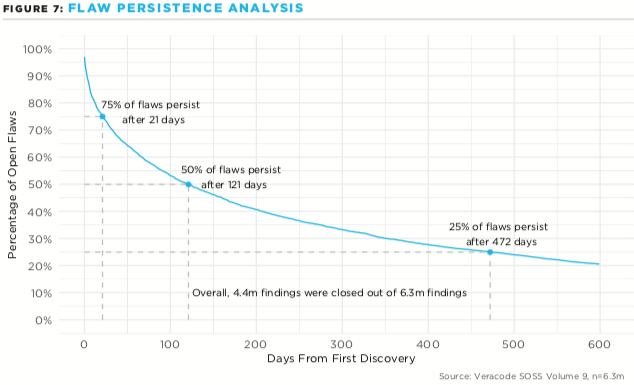
Notice how right away there is significant activity (the steep drop starting in the upper left) and how that leads to 25% of the findings being closed in first three weeks (21 days). However the next 25% of findings take a bit longer, and it takes a little over another 3 more months (121 days total) to see 50% of the findings closed. At this point the curve is starting to flatten out though, the rate of closures on the “old” findings is really slowing down, and the next 25% requires almost another year to address (472 days from discovery).
One challenge in communicating this analysis is that the results are a distribution of probability over time. Some organizations may start out strong and slow down while other orgs may start slow but catch up quick — it’s very difficult to capture those differences when reducing it down to a single comparable number. That’s why we chose to highlighting those three points on the curve. It enables us to compare the initial close rate (25%) with the median close rate (50%) with the long-game (75%) across different variables we will be looking at.
To illustrate those three points, let’s take a look at the close rates across industries: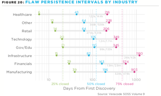 There is a whole lot being communicated in this plot, so let’s step through it. At a high-level, we’ve got the close rate for 25% (green), 50% (blue) and 75% (red) of the findings. Also, notice the horizontal axis is on a log scale: the closure rates have quite a long tail and if we were on a linear scale, the 25% numbers would look like they are all about the same time. So the log-scale gives us the ability to see differences at both ends. Also, notice that each of these intervals has some light gray text underneath at the right, this is stating how many closed/total findings were in that grouping. So Gov/Edu had about 99,000 findings closed out of about 133,000 findings, compared to the Technology sector which had 1.2 million closed out of 1.7 million (knowing the sample size in each slice is helpful if you speak that language). Finally, there are subtle dotted vertical lines for the three break points. These are communicating the overall rate of closures from the first plot: 21 days, 121 days and 472 days. This makes it easy to look at these industries and see which are better or worse than average for the three points.
It’s relatively easy to look across the sectors and compare the three different points taken from the survival plot. Take a look at the Infrastructure sector in the above plot. They do quite well off the starting block and close 25% of the findings in 15 days, and even 50% of the findings in 82 days. But for some reason, they slow way down after that, and take a whopping 1,180 days in the next timespan (about three years to from 50% closed to 75% closed). There must be something in that sector pushing for quick closures, maybe of the critical findings, but a lack of pushing after that, which causes that extremely long tail.
The full report looks at multiple different perspectives in flaw persistence such as the close rates across languages, severity, criticality and the effect of region and even internally developed versus open source (spoiler, internal apps fared better). I highly recommend reading the State of Software Security report from Veracode.